本篇主要实现一个神经网络并应用于CIFAR-10数据集。
计算损失函数与梯度
    W1, b1 = self.params['W1'], self.params['b1']
    W2, b2 = self.params['W2'], self.params['b2']
    N, D = X.shape

    # Compute the forward pass
    scores = None

    hidden_layer = np.maximum(0, np.dot(X, W1) + b1) #ReLU
    scores = np.dot(hidden_layer, W2) + b2
    # print scores

    # If the targets are not given then jump out, we're done
    if y is None:
      return scores

    # Compute the loss
    loss = None

    # visual prob
    exp_scores = np.exp(scores)
    probs = exp_scores / np.sum(exp_scores, axis=1, keepdims=True) # [N x K]

    #calculate loss
    corect_logprobs = -np.log(probs[range(N),y])
    data_loss = np.sum(corect_logprobs)/N
    reg_loss = 0.5*reg*np.sum(W1*W1) + 0.5*reg*np.sum(W2*W2)
    loss = data_loss + reg_loss

    # Backward pass: compute gradients
    grads = {}
    # calcute gradient
    dscores = probs
    dscores[range(N),y] -= 1
    dscores /= N

    # graident backforwar
    dW2 = np.dot(hidden_layer.T, dscores)
    db2 = np.sum(dscores, axis=0, keepdims=False)

    dhidden = np.dot(dscores, W2.T)

    dhidden[hidden_layer <= 0] = 0
    # get w b gradient
    dW1 = np.dot(X.T, dhidden)
    db1 = np.sum(dhidden, axis=0, keepdims=False)

    # add regular
    dW2 += reg * W2
    dW1 += reg * W1
    grads['W1']=dW1
    grads['W2']=dW2
    grads['b1']=db1
    grads['b2']=db2

    return loss, grads
检验损失函数与梯度
def rel_error(x, y):
  """ returns relative error """
  return np.max(np.abs(x - y) / (np.maximum(1e-8, np.abs(x) + np.abs(y))))

print 'Difference between your scores and correct scores:'
print np.sum(np.abs(scores - correct_scores))


loss, _ = net.loss(X, y, reg=0.1)
correct_loss = 1.30378789133

# should be very small, we get < 1e-12
print 'Difference between your loss and correct loss:'
print np.sum(np.abs(loss - correct_loss))

loss, grads = net.loss(X, y, reg=0.1)

# these should all be less than 1e-8 or so
for param_name in grads:

  f = lambda j: net.loss(X, y, reg=0.1)[0]
  #print type(f),type(net.loss(X, y, reg=0.1)[0])
  param_grad_num = eval_numerical_gradient(f, net.params[param_name], verbose=False)
  print '%s max relative error: %e' % (param_name, rel_error(param_grad_num, grads[param_name]))
训练神经网络
def train(self, X, y, X_val, y_val,
            learning_rate=1e-3, learning_rate_decay=0.95,
            reg=1e-5, num_iters=100,
            batch_size=200, verbose=False):
    num_train = X.shape[0]
    iterations_per_epoch = max(num_train / batch_size, 1)

    # Use SGD to optimize the parameters in self.model
    loss_history = []
    train_acc_history = []
    val_acc_history = []

    for it in xrange(num_iters):
      X_batch = None
      y_batch = None

      idx = np.random.choice(num_train, batch_size, replace=True)
      X_batch = X[idx]
      y_batch = y[idx]


      # Compute loss and gradients using the current minibatch
      loss, grads = self.loss(X_batch, y=y_batch, reg=reg)
      loss_history.append(loss)


      self.params['W1'] += -learning_rate * grads['W1']
      self.params['b1'] += -learning_rate * grads['b1']
      self.params['W2'] += -learning_rate * grads['W2']
      self.params['b2'] += -learning_rate * grads['b2']


      if verbose and it % 100 == 0:
        print 'iteration %d / %d: loss %f' % (it, num_iters, loss)

      # Every epoch, check train and val accuracy and decay learning rate.
      if it % iterations_per_epoch == 0:
        # Check accuracy
        train_acc = (self.predict(X_batch) == y_batch).mean()
        val_acc = (self.predict(X_val) == y_val).mean()
        train_acc_history.append(train_acc)
        val_acc_history.append(val_acc)

        # Decay learning rate
        learning_rate *= learning_rate_decay

    return {
      'loss_history': loss_history,
      'train_acc_history': train_acc_history,
      'val_acc_history': val_acc_history,
    }

def predict(self, X):
    y_pred = None


    hidden_layer = np.maximum(0, np.dot(X, self.params['W1']) + self.params['b1'])
    scores = np.dot(hidden_layer, self.params['W2']) + self.params['b2']
    y_pred = np.argmax(scores, axis=1)
    return y_pred
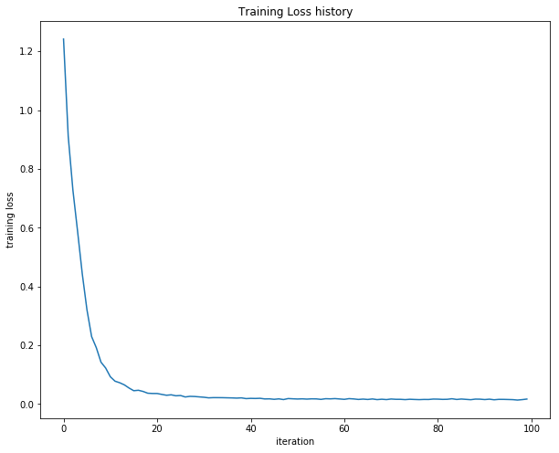
画出损失函数变化图
net = init_toy_model()
stats = net.train(X, y, X, y,
            learning_rate=1e-1, reg=1e-5,
            num_iters=100, verbose=False)

print 'Final training loss: ', stats['loss_history'][-1]

# plot the loss history
plt.plot(stats['loss_history'])
plt.xlabel('iteration')
plt.ylabel('training loss')
plt.title('Training Loss history')
plt.show()
导入CIFAR-10数据集
Train data shape:  (49000, 3072)
Train labels shape:  (49000,)
Validation data shape:  (1000, 3072)
Validation labels shape:  (1000,)
Test data shape:  (1000, 3072)
Test labels shape:  (1000,)
训练神经网络
这里我们将用SGD with momentum,学习率将会随着时间递减
input_size = 32 * 32 * 3
hidden_size = 50
num_classes = 10
net = TwoLayerNet(input_size, hidden_size, num_classes)

# Train the network
stats = net.train(X_train, y_train, X_val, y_val,
            num_iters=1000, batch_size=200,
            learning_rate=1e-4, learning_rate_decay=0.95,
            reg=0.5, verbose=True)

# Predict on the validation set
val_acc = (net.predict(X_val) == y_val).mean()
print 'Validation accuracy: ', val_acc
最后准确率可以达到28%左右
Debug the training
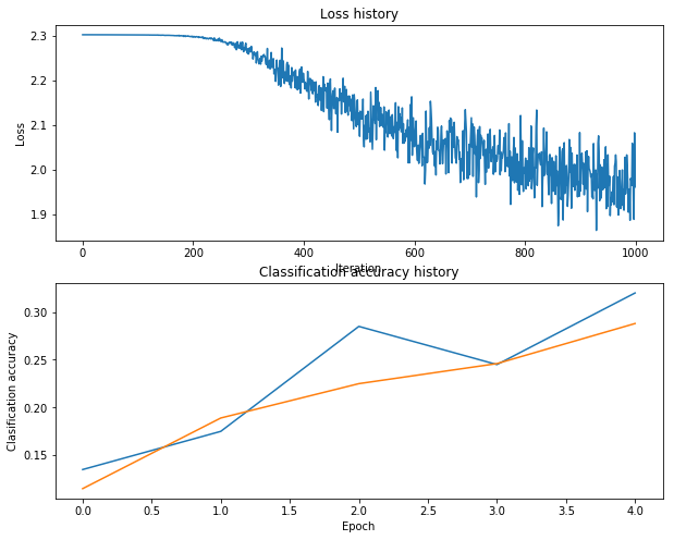
通过默认的参数,效果并不很好,只有28%左右,不是很好。
One strategy for getting insight into what’s wrong is to plot the loss function and the accuracies on the training and validation sets during optimization.
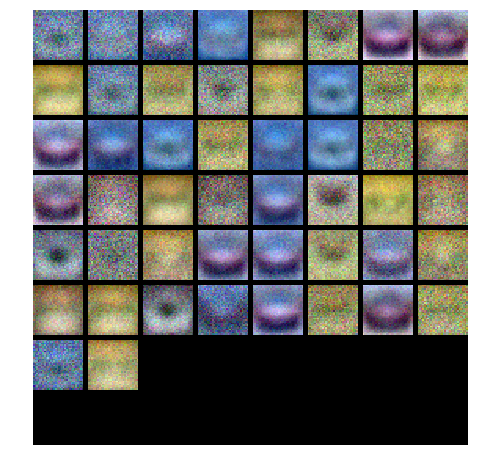
Another strategy is to visualize the weights that were learned in the first layer of the network. In most neural networks trained on visual data, the first layer weights typically show some visible structure when visualized.
# Plot the loss function and train / validation accuracies
plt.subplot(2, 1, 1)
plt.plot(stats['loss_history'])
plt.title('Loss history')
plt.xlabel('Iteration')
plt.ylabel('Loss')

plt.subplot(2, 1, 2)
plt.plot(stats['train_acc_history'], label='train')
plt.plot(stats['val_acc_history'], label='val')
plt.title('Classification accuracy history')
plt.xlabel('Epoch')
plt.ylabel('Clasification accuracy')
plt.show()
把权重可视化
def show_net_weights(net):
  W1 = net.params['W1']
  W1 = W1.reshape(32, 32, 3, -1).transpose(3, 0, 1, 2)
  plt.imshow(visualize_grid(W1, padding=3).astype('uint8'))
  plt.gca().axis('off')
  plt.show()

show_net_weights(net)
调整超参数
What’s wrong?. Looking at the visualizations above, we see that the loss is decreasing more or less linearly, which seems to suggest that the learning rate may be too low. Moreover, there is no gap between the training and validation accuracy, suggesting that the model we used has low capacity, and that we should increase its size. On the other hand, with a very large model we would expect to see more overfitting, which would manifest itself as a very large gap between the training and validation accuracy.
Tuning. Tuning the hyperparameters and developing intuition for how they affect the final performance is a large part of using Neural Networks, so we want you to get a lot of practice. Below, you should experiment with different values of the various hyperparameters, including hidden layer size, learning rate, numer of training epochs, and regularization strength. You might also consider tuning the learning rate decay, but you should be able to get good performance using the default value.
hidden_size = [75, 100, 125]

results = {}
best_val_acc = 0
best_net = None

learning_rates = np.array([0.7, 0.8, 0.9, 1, 1.1])*1e-3
regularization_strengths = [0.75, 1, 1.25]

print 'running',
for hs in hidden_size:
    for lr in learning_rates:
        for reg in regularization_strengths:
            print '.',
            net = TwoLayerNet(input_size, hs, num_classes)
            # Train the network
            stats = net.train(X_train, y_train, X_val, y_val,
            num_iters=1500, batch_size=200,
            learning_rate=lr, learning_rate_decay=0.95,
            reg= reg, verbose=False)
            val_acc = (net.predict(X_val) == y_val).mean()
            if val_acc > best_val_acc:
                best_val_acc = val_acc
                best_net = net
            results[(hs,lr,reg)] = val_acc
print
print "finshed"
# Print out results.
for hs,lr, reg in sorted(results):
    val_acc = results[(hs, lr, reg)]
    print 'hs %d lr %e reg %e val accuracy: %f' % (hs, lr, reg,  val_acc)

print 'best validation accuracy achieved during cross-validation: %f' % best_val_acc
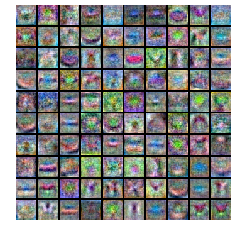
best validation accuracy achieved during cross-validation: 0.502000.
产生了50.2%的最好成绩
再可视化现在的weight
开始预测
test_acc = (best_net.predict(X_test) == y_test).mean()
print 'Test accuracy: ', test_acc
成功率超过50%