本文主要包括以下内容:
- implement a fully-vectorized loss function for the Softmax classifier
- implement the fully-vectorized expression for its analytic gradient
- check your implementation with numerical gradient
- use a validation set to tune the learning rate and regularization strength
- optimize the loss function with SGD
- visualize the final learned weights
计算损失函数
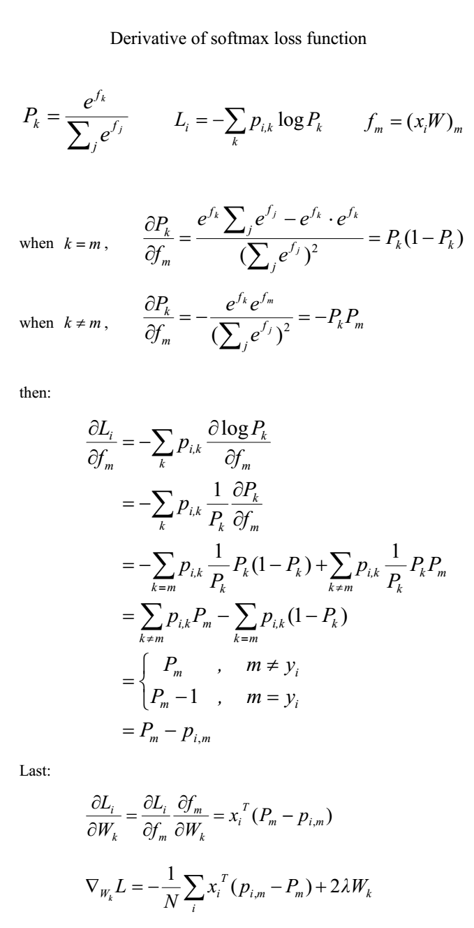
 详细可参见:Softmax损失函数及梯度的计算
def softmax_loss_naive(W, X, y, reg):
  loss = 0.0
  dW = np.zeros_like(W)
  f=np.dot(X,W)  #N*C
  fm=np.reshape(np.max(f,axis=1),(X.shape[0],1)) #N*1
  L = -np.log(np.exp(f-fm)/np.sum(np.exp(f-fm),axis=1,keepdims=True))
  for i in xrange(X.shape[0]):
    for j in xrange(W.shape[1]):
        if (y[i]==j):
            loss+=L[i,j]

  loss=loss/X.shape[0]
  loss+=0.5 * reg * np.sum(W * W)
  return loss, dW
在未经训练时,由于权重是随机生成的,因此应该每个分类的概率就是10%,因此 loss应该接近 -log (0.1)
计算梯度

加上梯度后的softmax_loss_naive版本:
  num_train = X.shape[0]
  num_classes = W.shape[1]
  f = X.dot(W)  #N by C
  f_max = np.reshape(np.max(f, axis = 1), (num_train, 1))
  prob = np.exp(f - f_max)/np.sum(np.exp(f-f_max), axis = 1, keepdims = True)

  for i in xrange(num_train):
    for j in xrange(num_classes):
        if (j == y[i]):
            loss += -np.log(prob[i,j])
            dW[:,j] += (1 - prob[i,j]) * X[i]
        else:
            dW[:,j] -= prob[i,j] * X[i]

  loss /= num_train
  loss += 0.5 * reg * np.sum(W*W)
  dW = -dW / num_train + reg * W
梯度校验
loss, grad = softmax_loss_naive(W, X_dev, y_dev, 0.0)

# As we did for the SVM, use numeric gradient checking as a debugging tool.
# The numeric gradient should be close to the analytic gradient.
from cs231n.gradient_check import grad_check_sparse
f = lambda w: softmax_loss_naive(w, X_dev, y_dev, 0.0)[0]
grad_numerical = grad_check_sparse(f, W, grad, 10)

# similar to SVM case, do another gradient check with regularization
loss, grad = softmax_loss_naive(W, X_dev, y_dev, 1e2)
f = lambda w: softmax_loss_naive(w, X_dev, y_dev, 1e2)[0]
grad_numerical = grad_check_sparse(f, W, grad, 10)
向量版实现
num_train = X.shape[0]
  num_classes = W.shape[1]
  f = X.dot(W)  #N by C
  f_max = np.reshape(np.max(f, axis = 1), (num_train, 1))
  prob = np.exp(f - f_max)/np.sum(np.exp(f-f_max), axis = 1, keepdims = True)

  keepProb = np.zeros_like(prob)
  keepProb[np.arange(num_train), y] = 1.0
  loss += -np.sum(keepProb * np.log(prob)) / num_train + 0.5 * reg * np.sum(W*W)
  dW += -np.dot(X.T, keepProb - prob)/num_train + reg * W
通过交叉验证以获得超参数
for lr in learning_rates:
    for rs in regularization_strengths:
        print 'Trying learning rate as %f, regularization strength as %f' % (lr, rs)  #01
        softmax = Softmax()
        softmax.train(X_train, y_train, learning_rate=lr, reg=rs,
                      num_iters=1500, verbose=True)

        y_train_pred = softmax.predict(X_train)
        training_accuracy = np.mean(y_train == y_train_pred)

        y_val_pred = softmax.predict(X_val)
        val_accuracy = np.mean(y_val == y_val_pred)

        results[(lr, rs)] = (training_accuracy, val_accuracy)

        if val_accuracy > best_val:
            best_val = val_accuracy
            best_softmax = softmax
最后产生的正确率在35%左右,在测试集上的正确率为0.337000
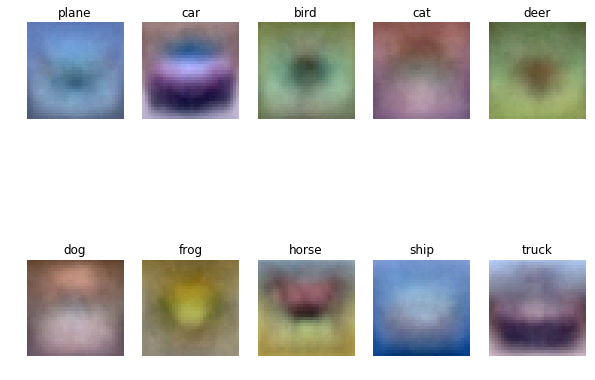
可视化权重
w = best_softmax.W[:-1,:] # strip out the bias
w = w.reshape(32, 32, 3, 10)

w_min, w_max = np.min(w), np.max(w)

classes = ['plane', 'car', 'bird', 'cat', 'deer', 'dog', 'frog', 'horse', 'ship', 'truck']
for i in xrange(10):
  plt.subplot(2, 5, i + 1)

  # Rescale the weights to be between 0 and 255
  wimg = 255.0 * (w[:, :, :, i].squeeze() - w_min) / (w_max - w_min)
  plt.imshow(wimg.astype('uint8'))
  plt.axis('off')
  plt.title(classes[i])
W中的每一个分类对应的数值(维度为D的数组,D = 32 * 32 * 3),本质是就是这个分类中所有图像的像素值的综合,因而将它还原成图像后,你会发现它就是它所代表的分类的图像。
