本作业的目标如下:
- implement a fully-vectorized loss function for the SVM
- implement the fully-vectorized expression for its analytic gradient
- check your implementation using numerical gradient
- use a validation set to tune the learning rate and regularization strength
- optimize the loss function with SGD
- visualize the final learned weights
归一化图片
mean_image = np.mean(X_train, axis=0)
print mean_image[:10] # print a few of the elements
plt.figure(figsize=(4,4))
plt.imshow(mean_image.reshape((32,32,3)).astype('uint8')) # visualize the mean image
plt.show()
X_train -= mean_image
X_val -= mean_image
X_test -= mean_image
X_dev -= mean_image
损失函数与梯度计算
def svm_loss_naive(W, X, y, reg):
  dW = np.zeros(W.shape) # initialize the gradient as zero

  # compute the loss and the gradient
  num_classes = W.shape[1]
  num_train = X.shape[0]
  loss = 0.0
  for i in xrange(num_train):
    scores = X[i].dot(W)
    correct_class_score = scores[y[i]]
    for j in xrange(num_classes):
      if j == y[i]:
        continue
      margin = scores[j] - correct_class_score + 1 # note delta = 1

      if margin > 0:
        loss += margin
        dW[:, y[i]] += -X[i, :]     # compute the correct_class gradients
        dW[:, j] += X[i, :]         # compute the wrong_class gradients
  # Right now the loss is a sum over all training examples, but we want it
  # to be an average instead so we divide by num_train.
  loss /= num_train
  dW /= num_train
  dW += 2 * reg * W

  # Add regularization to the loss.
  loss += 0.5 * reg * np.sum(W * W)

  return loss, dW
关于梯度的计算:详情可参见SVM损失函数及梯度矩阵的计算
梯度检验
def grad_check_sparse(f, x, analytic_grad, num_checks=10, h=1e-5):
  """
  sample a few random elements and only return numerical
  in this dimensions.
  """

  for i in xrange(num_checks):
    ix = tuple([randrange(m) for m in x.shape])

    oldval = x[ix]
    x[ix] = oldval + h # increment by h
    fxph = f(x) # evaluate f(x + h)
    x[ix] = oldval - h # increment by h
    fxmh = f(x) # evaluate f(x - h)
    x[ix] = oldval # reset

    grad_numerical = (fxph - fxmh) / (2 * h)
    grad_analytic = analytic_grad[ix]
    rel_error = abs(grad_numerical - grad_analytic) / (abs(grad_numerical) + abs(grad_analytic))
    print 'numerical: %f analytic: %f, relative error: %e' % (grad_numerical, grad_analytic, rel_error)


from cs231n.gradient_check import grad_check_sparse
f = lambda w: svm_loss_naive(w, X_dev, y_dev, 0.0)[0]
grad_numerical = grad_check_sparse(f, W, grad)

# do the gradient check once again with regularization turned on
# you didn't forget the regularization gradient did you?
loss, grad = svm_loss_naive(W, X_dev, y_dev, 1e2)
f = lambda w: svm_loss_naive(w, X_dev, y_dev, 1e2)[0]
grad_numerical = grad_check_sparse(f, W, grad)
使用向量化方法计算损失函数与梯度
def svm_loss_vectorized(W, X, y, reg):

  loss = 0.0
  dW = np.zeros(W.shape) # initialize the gradient as zero


  scores = X.dot(W)  # N by C
  num_train = X.shape[0]
  num_classes = W.shape[1]
  scores_correct = scores[np.arange(num_train), y] #1 by N
  scores_correct = np.reshape(scores_correct, (num_train, 1)) # N by 1
  margins = scores - scores_correct + 1.0 # N by C
  margins[np.arange(num_train), y] = 0.0
  margins[margins <= 0] = 0.0
  loss += np.sum(margins) / num_train
  loss += 0.5 * reg * np.sum(W * W)

  margins[margins > 0] = 1.0                         #
  row_sum = np.sum(margins, axis=1)                  # 1 by N
  margins[np.arange(num_train), y] = -row_sum
  dW += np.dot(X.T, margins)/num_train + reg * W     # D by C

  return loss, dW
随机梯度下降
 def train(self, X, y, learning_rate=1e-3, reg=1e-5, num_iters=100,
                          batch_size=200, verbose=True):
        num_train, dim = X.shape
        # assume y takes values 0...K-1 where K is number of classes
        num_classes = np.max(y) + 1
        if self.W is None:
            # lazily initialize W
            self.W = 0.001 * np.random.randn(dim, num_classes)   # D by C

        # Run stochastic gradient descent(Mini-Batch) to optimize W
        loss_history = []
        for it in xrange(num_iters):
            X_batch = None
            y_batch = None
            # Sampling with replacement is faster than sampling without replacement.
            sample_index = np.random.choice(num_train, batch_size, replace=False)
            X_batch = X[sample_index, :]   # batch_size by D
            y_batch = y[sample_index]      # 1 by batch_size
            # evaluate loss and gradient
            loss, grad = self.loss(X_batch, y_batch, reg)
            loss_history.append(loss)

            # perform parameter update
            self.W += -learning_rate * grad
            if verbose and it % 100 == 0:
                print 'Iteration %d / %d: loss %f' % (it, num_iters, loss)

        return loss_history
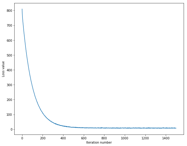
随着梯度下降过程中,损失函数的变化
# A useful debugging strategy is to plot the loss as a function of
# iteration number:
plt.plot(loss_hist)
plt.xlabel('Iteration number')
plt.ylabel('Loss value')
plt.show()
预测
def predict(self, X):

    #print X.shape,self.W.shape

    scores = X.dot(self.W)
    y_pred = np.argmax(scores, axis = 1)
    return y_pred
validation验证集
learning_rates = [1.4e-7, 1.5e-7, 1.6e-7]
regularization_strengths = [(1+i*0.1)*1e4 for i in range(-3,3)] + [(2+0.1*i)*1e4 for i in range(-3,3)]

results = {}
best_val = -1   # The highest validation accuracy that we have seen so far.
best_svm = None # The LinearSVM object that achieved the highest validation rate.


for rs in regularization_strengths:
    for lr in learning_rates:
        svm = LinearSVM()
        loss_hist = svm.train(X_train, y_train, lr, rs, num_iters=3000)
        y_train_pred = svm.predict(X_train)
        train_accuracy = np.mean(y_train == y_train_pred)
        y_val_pred = svm.predict(X_val)
        val_accuracy = np.mean(y_val == y_val_pred)
        if val_accuracy > best_val:
            best_val = val_accuracy
            best_svm = svm
        results[(lr,rs)] = train_accuracy, val_accuracy


# Print out results.
for lr, reg in sorted(results):
    train_accuracy, val_accuracy = results[(lr, reg)]
    print 'lr %e reg %e train accuracy: %f val accuracy: %f' % (
                lr, reg, train_accuracy, val_accuracy)

print 'best validation accuracy achieved during cross-validation: %f' % best_val
可视化cross-validation结果
import math
x_scatter = [math.log10(x[0]) for x in results]
y_scatter = [math.log10(x[1]) for x in results]

# plot training accuracy
marker_size = 100
colors = [results[x][0] for x in results]
plt.subplot(2, 1, 1)
plt.scatter(x_scatter, y_scatter, marker_size, c=colors)
plt.colorbar()
plt.xlabel('log learning rate')
plt.ylabel('log regularization strength')
plt.title('CIFAR-10 training accuracy')

# plot validation accuracy
colors = [results[x][1] for x in results] # default size of markers is 20
plt.subplot(2, 1, 2)
plt.scatter(x_scatter, y_scatter, marker_size, c=colors)
plt.colorbar()
plt.xlabel('log learning rate')
plt.ylabel('log regularization strength')
plt.title('CIFAR-10 validation accuracy')
plt.show()
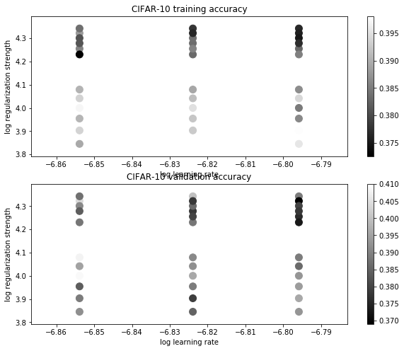
将所得bestSVM应用于测试集,结果为 0.381000
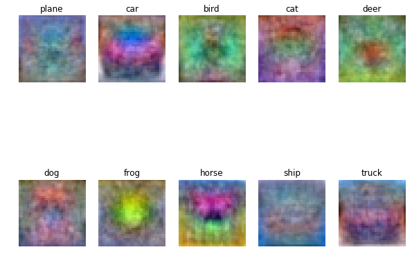
可视化wight各图片成分
w = best_svm.W[:-1,:] # strip out the bias
w = w.reshape(32, 32, 3, 10)
w_min, w_max = np.min(w), np.max(w)
classes = ['plane', 'car', 'bird', 'cat', 'deer', 'dog', 'frog', 'horse', 'ship', 'truck']
for i in xrange(10):
  plt.subplot(2, 5, i + 1)

  # Rescale the weights to be between 0 and 255
  wimg = 255.0 * (w[:, :, :, i].squeeze() - w_min) / (w_max - w_min)
  plt.imshow(wimg.astype('uint8'))
  plt.axis('off')
  plt.title(classes[i])